What's Your Mean?
Problem
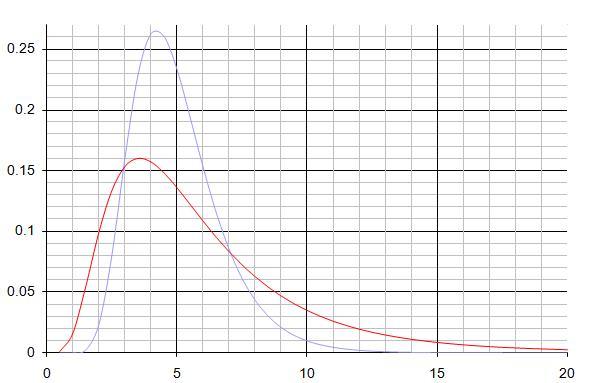
The probability density functions for two related, but unknown, distributions are given in the following accurately plotted chart.
It is known that the means of the distributions are whole numbers, and that the two pdfs only have a single turning point.
By numerically estimating the required integrals, what can you deduce with certainty about the two means?

Getting Started
Although numerical integration is not exact, you might like to try to do a numerical integration which you KNOW is smaller than the mean and then do another integration which you can be very sure gives a value which is larger than the mean.
Don't forget that you can break an area down into rectangles or trapezia.
Student Solutions
Probability Density Functions
The probability density function, or PDF, is a function which describes the probability of a random variable taking on certain values. For a continuous random variable, the probability that the variable lies between two values is given by the integral of the density function between these values.
We know that the sum of the probabilities of all possible outcomes is 1. So the integral of the PDF over all possible values of the variable is equal to 1.
We also need to know how to calculate the mean of the variable from the PDF. We first recall the definition of mean: $ \bar{x}=\Sigma x \,Pr(\hbox{X=x})$
Because the integral of the PDF gives us the probabilities of the variable occuring, the equation for the mean becomes $$ \bar{x}=\int xf(x) \,dx $$ where $f(x)$ is the density function.
Integrating using area approximation
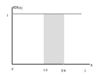
For example, consider a variable with the distribution function as below.
We wish to calculate $ Pr(1/2 \leq X \leq 3/4) $ which we can find by calculating the area of the shaded rectangle:
$$ Pr(1/2 \leq X \leq 3/4) =\int^{3/4}_{1/2} \,dx= base \times height = ({3\over 4} - {1\over 2}) \times 1 = {1\over 4} $$
Red Line Mean
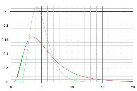
Applying the same idea to the red line in the problem, we can estimate the area under the curves using rectangles and trapeziums. Two such trapeziums are marked below in green.
To find the area of the trapezium, we use the result $ Area(trapezium) = {h \times (a+b) \over 2} $
This gives us the probability that our variable lies within the small trapezium of height 1. To find the mean, we then need to multiply this probability by the value of the variable in this interval. We approximate here, by using the midpoint of the trapezium height.
Take for example the above trapezium on the right, where the variable ranges from 10 to 11. We approximate by taking the value of the variable as 10.5, and mutiply this by the probability of the region to get the mean. The table below gives our estimates of these values.
| h= | a= | b= | Area | Midpoint | Mean |
| 0.5 | 0 | 0.01 | 0.005 | 0.75 | 0.00375 |
| 1 | 0.015 | 0.1 | 0.0575 | 1.5 | 0.08625 |
| 1 | 0.1 | 0.15 | 0.0125 | 2.5 | 0.3125 |
| 1 | 0.15 | 0.155 | 0.1525 | 3.5 | 0.53375 |
| 1 | 0.155 | 0.135 | 0.145 | 4.5 | 0.6525 |
| 1 | 0.135 | 0.12 | 0.1275 | 5.5 | 0.70125 |
| 1 | 0.12 | 0.085 | 0.1025 | 6.5 | 0.66625 |
| 1 | 0.085 | 0.06 | 0.0725 | 7.5 | 0.54375 |
| 1 | 0.06 | 0.045 | 0.0525 | 8.5 | 0.44625 |
| 1 | 0.045 | 0.035 | 0.04 | 9.5 | 0.38 |
| 1 | 0.035 | 0.025 | 0.03 | 10.5 | 0.315 |
| 1 | 0.025 | 0.02 | 0.0225 | 11.5 | 0.25875 |
| 1 | 0.02 | 0.015 | 0.0175 | 12.5 | 0.21875 |
| 1 | 0.015 | 0.01 | 0.0125 | 13.5 | 0.16875 |
| 1 | 0.01 | 0.01 | 0.01 | 14.5 | 0.145 |
The sum of the means in the right hand column is 5.4325. Because the question tells us the mean is an integer, we should also approximate the mean in the region 15 to 20.
As the probabilities in this range are so low, it is easier to approximate the area as a very flat rectangle. Remembering that the area under the PDF is the same as the probability of the variable being in that region, we find $$ Pr(15 \leq X \leq 20)=5 \times 0.005=0.025 $$ Again we use the midpoint approximation, and find $$ \bar{x}=17.5 \times 0.025 = 0.4375 $$
Summing over all the means, this gives us $ \bar{x}=5.4325 + 0.4375 = 5.87 \approx 6 $
We leave the grey line for you to compute. You might want to find an even closer estimation of the mean, and then find the relationship between the two PDFs.
Teachers' Resources
Using NRICH Tasks Richly describes ways in which teachers and learners can work with NRICH tasks in the classroom.
