Population dynamics - part 2

Discrete Modelling

We often use discrete mathematics to model a population when time is modelled in discrete steps. This fits well with annual censuses of wildlife populations. 

Sometimes populations are themselves discrete, such as:

• Species with non-overlapping generations (eg. annual plants)
• Species with pulsed reproductions (eg. many wildlife species in seasonal environments)

Geometric Growth

The population equation, $N_{t+1}=\lambda N_t$ , from before means that over discrete intervals of time,$t_0, t_1, t_2, ...$, the rate of change in population size is proportional to the size of the population.

We first solve this equation: $$\begin{align*} N_{t+1}&=\lambda N_t \\ &=\lambda \lambda N_{t-1} \\& =...\\ &= \lambda^{t+1} N_0 \\ \Rightarrow N_t &=\lambda^t N_0 \end{align*}$$ The population size will depend on the value of $\lambda$

• If $\lambda> 1$ then exponential increase
• If $\lambda=1$ then stationary population
• If $\lambda< 1$ then exponential decrease

Question:  If a population of owls increases by 40% in a year, what is the value of r and $\lambda$ ?

Given there were initially 10 owls, what will the population size be in 75 days?  Can you plot this population growth?

Exponential Growth

Some populations may grow continuously, without pulsed births and deaths (eg. humans). In these cases, time is a continuous smooth curve, so we use differential equations to represent this continuous model.

Using our discrete model from above: $$\begin{align*} N_{t+\Delta t}&=\lambda^{\Delta t} N_t =(1+r)^{\Delta t}N(t)\approx (1+r\Delta t) N(t)\\  \Rightarrow \Delta N_t&\approx r \Delta t N_t \\  \\\Rightarrow \lim_{\Delta t \to 0} \frac{\Delta N(t)}{\Delta t} &=\frac {\mathrm{d}N(t)}{\mathrm{d}t}=rN(t) \end{align*}$$ Question:  Solve the equation, $\frac {\mathrm{d}N(t)}{\mathrm{d}t}=rN(t)$ , using standard integrals, showing that the solution is $N(t)=N_0e^{rt}$.

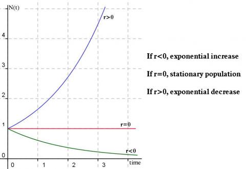
Different values of r determine the change in population size, as shown below.

Image

Also note the connection between the discrete and continous solutions:  $$\begin{align*} N_t =\lambda^t N_0  &\text{  and  }  N(t)=N_0 e^{rt} \\ \Rightarrow \lambda^t&=e^{rt} \\ \lambda&=e^r \\ \ln(\lambda)&=r \end{align*}$$ Question:  Using the discrete model above, how long does it take for this population to double in size? What about the continous case?

Limitations of the Models

Consider a population of insects which suddenly dies out right before the start of every time period, and whose children hatch right after. A discrete model would lead us to believe that there are no insects during the entire period, so instead we should use a continuous model.

On the other hand, it is often impossible to continually monitor the population size, so we approximate using the discrete case.

Choosing which of discrete or continuous to use is an important decision in modelling populations.

Can you also think of any assumptions we have made with these models, and why they could be a problem? Consider the environment the population inhabits and differences between members of the population.

Click here to see the geometric model adapted to include environmental resistance.

Question:  If $\lambda = 1.25$, by how much does a population of blue footed boobies increase per year?

The population N(t) of blue footed boobies is assumed to satisfy the logistic growth equation $\frac {\mathrm{d}N}{\mathrm{d}t}=\frac{1}{500} N(t) \big( 1-N(t)\big)$ . Given $N_0=200$, solve for N(t). Repeat for $N_0=2000$. Discuss the long-term behaviour of the population in both cases.