Suppose we want a cell, that has numbers in blue, to switch to red
type if that cell value becomes negative.
Make sure that the correct cell is selected.
From the Format menu choose conditional formatting . . . and a dialogue box will appear.


Make the cell become negative, then positive, then 0, etc. Checking that the conditional formatting is triggered correctly.
More Powerful Conditions
It can often be very useful for the format change to trigger on a calculated value not a specified value.
In the More Beads sheet I set conditional formatting to trigger if a cell matched its integer part, that is had no fractional part.

Make sure that the correct cell is selected.
From the Format menu choose conditional formatting . . . and a dialogue box will appear.
Image

- Set the condition Cell Value Is to be less than 0 as shown in the illustration.
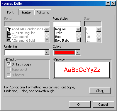
- Click the Format button on the dialogue box to set the appearance that the cell is to have if the condition is met.
Image

- Notice the limited range of format change that is possible. You can only set the font colour, the fill (background) colour, and the cell border colour.
- Click OK, and then OK back on the Condition box.
Make the cell become negative, then positive, then 0, etc. Checking that the conditional formatting is triggered correctly.
More Powerful Conditions
It can often be very useful for the format change to trigger on a calculated value not a specified value.
In the More Beads sheet I set conditional formatting to trigger if a cell matched its integer part, that is had no fractional part.
Image

- I changed the second input box from " between " to " equal to ".
- Typed in =INT(A2) in the third input box. The = is necessary because a calculation is required.
- Clicked the Format . . . button and made my choice, etc.
Note
When a cell is replicated, not only
its formula but also its formatting is copied. This includes
conditional formatting.
Experiment with these options.
