Population Dynamics - part 5

The Lotka-Volterra Equations

The Lotka-Volterra equations allow us to model a biological system containing a predator and a prey species. They arose in the 1920s due to the independent work of the mathematicians Alfred Lotka and Vito Volterra.

Formulating the Equations

Let x be the size of a fish population and y be the size of the shark population. If the prey have an unlimited food supply and no predators, then they grow exponentially according to the equation $\frac {\mathrm{d}x}{\mathrm{d}t}=\lambda x$ , for some constant $\lambda$.

If there are more sharks, more fish will be killed and if there are fewer sharks, then fewer fish will be killed.  So the rate of predation upon the prey is proportional to the rate at which the predators and prey meet. We represent this by $\alpha xy$.

Note that if either x or y is zero then there can be no predation.

The equation for prey becomes: $$\frac {\mathrm{d}x}{\mathrm{d}t}=\lambda x-\alpha xy =x(\lambda -\alpha y)$$ Conversely, predators rely on prey to survive, so in the absence of any prey, the predator equation is   $\frac {\mathrm{d}y}{\mathrm{d}t}=-\gamma y$.  The growth of the predator population will depend on the population sizes of the predators and prey, and the ability of the predators to successfully catch prey. We represent this by $\beta xy$.

The equation for predators becomes: $$\frac {\mathrm{d}y}{\mathrm{d}t}=\beta xy-\gamma y =y(\beta x -\gamma)$$

Using the Equations

We are interested in population equilibrium, which occurs when neither population is changing: $$ \begin{align*} \frac {\mathrm{d}x}{\mathrm{d}t}&=\frac {\mathrm{d}y}{\mathrm{d}t}=0 \\ x(\lambda -\alpha y)&=y(\beta x -\gamma)=0 \\ \Rightarrow x=0,y=0 &\text{  and  }  x=\frac{\gamma}{\beta}, y=\frac{\lambda}{\alpha} \end{align*}$$ The first solution occurs when both species die out, the second when the sizes of both species reach an equilibrium with each other.

Determining the stability of these equations, requires knowledge of the Jacobian matrix and linearization, which we exclude for complexity.

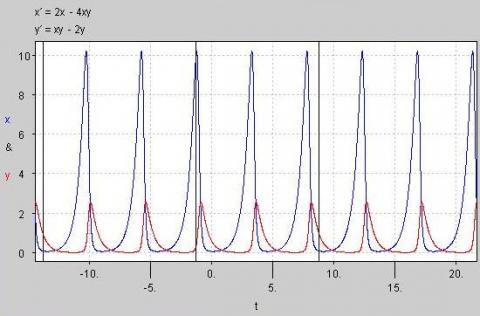
Question:  Consider a species of fish, x, and a species of shark, y, with population equations: $$\frac {\mathrm{d}x}{\mathrm{d}t}=2x-4xy ,    \frac {\mathrm{d}y}{\mathrm{d}t}=xy-2y$$ a) Where are the equilibrium points?

b) Below is a phasor diagram of the above equations. Try and work out what it is representing. What happens at the red point?

Image

We can also plot the size of the populations against time on the same graph. The graph below clearly shows the dependency of the shark population on a large population of prey, and the oscillatory nature of the two population sizes.

Image

Question:   Why do you think the shark population peaks after the fish population has soared? Why do you think the shark population is always less than the fish population?

Limitations to our model

In reality if two species coexist, their interactions also depend on the environment they inhabit. This is explored further here. Some of the assumptions made in the above equations are:

• The prey always find ample food
• The rate of change of population is proportional to its size

Question:   Can you think of any other assumptions we have made in our model?