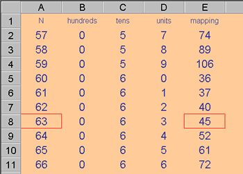
These notes explain a particular use of spreadsheets: looking up results which have already been calculated. There is quite a collection of Lookup functions available, but VLOOKUP (used in the Happy Numbers investigation) is the main topic here.
VLOOKUP: Looks down the first column of a block (range) for a specified value, then returns a value further along that same row.

For example:
= VLOOKUP (63, A1: E11, 5)
would look down the first column of the range A1: E11 until 63 was located, then return the value in that same row but in the fifth column.
The V of VLOOKUP stands for vertical. HLOOKUP performs the same process horizontally. HLOOKUP finds the position of a given value in the first row then, from the same column as the located value, returns the corresponding value from a specified lower row.
Two more Lookup functions deserve a brief mention:
INDEX and MATCH INDEX returns the value at a specific position in a given range.
= INDEX ( B6 : D10, 3, 2)
would return the value in the third row and second column of the range B6 : D10. This can be useful when the row and column values are variables.
MATCH
operates on a single row or on a single column. It returns the values position along that row or column.
= MATCH ( 63, A2 : A11, 0 )
would report that 63 was the seventh item in that line of values, A2 : A11 The 0 following the range reference, causes only an exact match to be reported.
