I used the linear programming interactivity with students on a Mathematics Enhancement Course. The Mathematics Enhancement Course comprises several five-week modules covering various topics within the A-level and undergraduate mathematics curriculum.
The linear programming interactivity was used in the first lesson of the Decision and Discrete module where most students were meeting linear programming for the first time. A few students had already covered this topic in A-level mathematics.
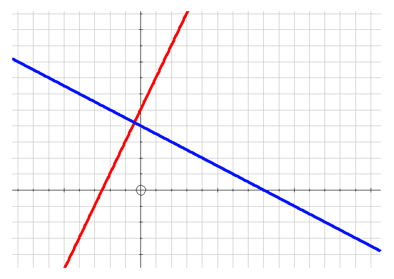
The session was held in a computer laboratory to allow hands on use of the linear programming interactivity. I used a PowerPoint presentation to guide the session. I started by checking students’ familiarity with using graphs to represent and solve simultaneous linear equations and defining regions using linear inequalities. Students used Autograph to solve the simultaneous equations y = 2x + 5 and 2y + x = 8. They also determined the linear inequalities that defined the various regions on the same graph.
This region (which includes the red and blue lines and the y-axis as boundaries) is defined by three linear inequalities y ≥ 0, 2y + x ≥ 8 and y ≤ 2x + 5:
Once students were confident with this prerequisite knowledge I introduced the linear programming interactivity in the Google Chrome browser. The web link was made available in the university VLE, Moodle. I asked students not to tick the feasible region option in order that they could figure out the feasible region for themselves.
Students worked through the questions available on the linear programming interactivity (questions 1-6) and then plotted the constraint lines. By interacting with the plotted graph they answered questions 7 and 8 and two additional questions:
They then tackled question 9 in the simulation to optimise the profit. Students were then encouraged to vary the original constraints and investigate how the feasible region changes. They learned how to solve the linear programming problem by using a sliding rule to represent the profit line or by evaluating the profit for extreme points of the feasible region.
The linear programming interactivity has the following problem:
Woods, Inc. is a toy manufacturer. Currently it manufactures wooden dolls and wooden trains. The current number of carpentry hours available per day at Woods, Inc. is 100 hours. Dolls usually take about 1 hour of carpentry whilst trains take about 2 hours. The time it takes to paint these toys is similar, i.e. 1 hour each, but there are only 80 painting hours available per day. Wooden trains are not the biggest seller and hence Woods, Inc. tries to keep the manufacturing of wooden trains to be 40 or less per day. Currently, dolls sell for £1 whilst the wooden trains sell for £2. Let the number of trains be and the number of wooden toys be . Given these constraints how can Woods, Inc. maximise profit?
Students were quick to identify the feasible region describing it as “The area where the constraints all apply at the same time.” They were pleased to see that the feasible region could be displayed automatically.

Some students struggled with:
7. What is the minimum number of dolls and trains that can be produced? Why? Where is this point located on the graph?
and needed to be reminded about the practical context:
Tutor: “Think in real-life now, if I had a toy factory and I was producing the dolls and trains, what is the minimum number of toys can I produce?”
Student: “Zero.”
Tutor: “Good! And where will that point be on the graph?”
Student: “At the origin!”
The students then worked on optimising the profit. When asked where the best profit occurred some students noticed,
Student: “It is where the lines intersect.”
Tutor: “Do you think it is always where the constraint lines intersect?”
Student: “Yes, I think so”
Tutor: “How do you know which intersection is correct? Why don’t you change your constraints and see if that is always the case?”
The students then experimented by varying the constraints and optimising the profit in each case. Many could justify the approach of using a sliding rule to represent the profit line or by evaluating the profit for extreme points of the feasible region in order to optimise the profit for any set of constraints.
Overall, I thought the session went well and the learning was more effective than with other approaches I’ve used. Students commented that they found the interactivity easier to use than Autograph and liked being able to see the feasible region. They liked being able to drag the constraint lines and explore how changing the constraints impacts the profit.