A large company has several warehouses, each having different amounts of stock of each item, which they need to distribute to their shops. They need to get the stock to to the shops as quickly as possible, and so need to work out the best method for this to happen. Or imagine you are a farmer, who has bought a certain amount of fertiliser and insecticide and a certain area of land which you can plant with some combination of Wheat and Barley. Wheat and Barley require different amounts of fertiliser and insecticide, but you have only a limited amount. How would you maximize your profits?

These problems are examples of linear programming problem, and can be solved using the Simplex Algorithm. The Simplex Algorithm starts by picking any valid solution (so the farmer not planting anything at all on his land is a perfectly valid solution, although he won't make much profit!), then at each stage moving to a better, more profitable solution. Finally, we arrive at a solution which is the most profitable.

Lets have a look at a simple example, which we are able to solve both with and without the simplex algorithm:
Maximise

x + y

subject to:

x + 2 y \leq 2

2 x + y \leq 3

x \geq 0

y \geq 0

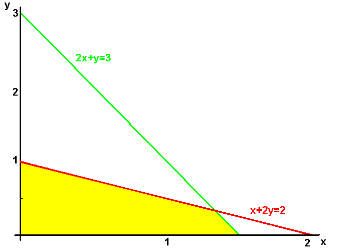
We can draw a graph in the x-y plane to show the valid range of x and y:

We want to maximise x+y, and we can do this by drawing a line x+y=constant, and if it intersects with the valid area we now have, then we can pick x and y in this and get our solution. So the best line can be drawn for c being 5/3, and here we get x=4/3 and y=1/3. Do you notice that this point is at a 'corner' of our valid area, at the intersection of the red and green lines? This isn't just a coincidence. If you look at the diagram, and draw a line x+y=c, for the biggest c possible, then either it will meet a line parallel to it, or it will meet a corner. So if we just look at the corner solutions, one of them will give us the maximum.

So if we can solve the problem just by drawing a couple of lines, why do we need this simplex algorithm? The problem above has just got two variables, x and y, so we can draw it (and often with only a few variables, drawing it is quicker!). If it had three variables, x, y and z, then you could probably make a model. But what happens if you have 4 or more variables? You can't draw it! So we need a different way of solving these problems - the simplex algorithm.

Remember that a maximum solution will always be at a corner? In the simplex algorithm we can take advantage of this by starting at one of these points, and then move along the edge to another point, always moving along a line that increases the function we wish to maximise.

Our problem contains inequalities, which are qute difficult to manipulate. To get around this by adding some extra variables, called slack variables. This is since if

x \geq c

then this is the same as always being about to find some

z \geq 0

so that x+z=c. It is also easier to call

x

x_{1}

and

y

y_{2}

, so we instead get the new equations:

Maximize $x_{1} + x_{2}$ subject to
$x_{1} + 2 x_{2} + z_{1} = 2$
$2 x_{1} + x_{2} + z_{2} = 3$
$x_{1} \geq 0$ , $x_{2} \geq 0$ , $z_{1} \geq 0$ , $z_{2} \geq 0$

We find that the solution being at a corner means that the number of variables (4) minus the number of constraint equatinos (2) is exactly the number of variables that are zero (2). So we start with the solution $x_{1} = x_{2} = 0$ , and so $z_{1} = 2$ and $z_{2} = 3$ . We now want to find a better solution. To do this we are going to make one of the $z$ 's zero and increase the value of one of the $x$ 's. We do this by getting the equations so that each of them only appear in one of the conditions, their coefficient is 1, and the left hand side is positive. We can then set everything else to 0 and find their values. We can pick any variable that is still positive in the original equation to increase, so lets choose $x_{1}$ , and then we choose which $z$ to remove by divinding each equation by the coefficient of $x_{1}$ , which equation has the smallest right hand side (this will prevent the right hand side of the equations from becoming negative). This is the second equation, so we choose $z_{2}$ . Doing this we get $x_{1} = 1.5$ , $z_{1} = 0.5$ , $x_{2} = z_{2} = 0$ . 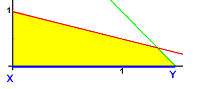So we have moved from point X to point Y on the graph:

plot, with the point we are now at, labelled Y
The re-written problem is:

Maximize $\frac{3}{2} + \frac{x_{2}}{2} - \frac{z_{2}}{2}$ subject to:
$\frac{3 x_{2}}{2} - \frac{z_{2}}{2} + z_{1} = \frac{1}{2}$
$\frac{x_{2}}{2} + \frac{z_{2}}{2} + x_{1} = \frac{3}{2}$
$x_{i} \geq 0$

So our function is now 1.5, so we are making some progress! If we increase $z_{2}$ , we will only decrease the function. So we will try to increase the value of $x_{2}$ , decreasing the value of $z_{1}$ . So we can make $x_{2} = 1 / 3$ , and so $x_{1} = 4 / 3$ , and $z_{1} = z_{2} = 0 .$ Now if we rearrange the equations again we get:

Maximize $5 / 3 - z_{1} / 3 - z_{2} / 3$ Subject to:
$2 z_{1} / 3 - z_{2} / 3 + x_{2} = 1 / 3$
$- z_{1} / 3 + 2 z_{2} / 3 + x_{1} = 4 / 3$

But the value is at its maximum when z_1 and z_2 are both zero, which they are, so the maximum is 5/3, and so we have found our the same answer as we had in our diagram, we have moved from point Y to the optimal solution at point Z:

But writing out all those

x_{1}

's and

x_{2}

's again and again isn't terribly convenient. This is why we have come up with a more convenient way of notating this - the Simplex Tableau:

Here we write each line of the equation by just writing their entries in the grid. Also notice that our variables which are non-zero (

z_{1}

and

z_{2}

) are only in one equation each. The simplex algorithm keeps this true for each table.

Earlier we picked a variable to increase whose coefficient was greater than zero, and so we would increase the maximum. So, lets pick the first column, doing the same as before.

Next, for each row we look at the final column and divide it by the entry in the column we picked (so in this case the first column). Pick the row where this value is smallest. This is done since after the next stage, we want the right hand side of the equation to be positive, and picking this ensures this. Now divide the whole row by the value in the column we chose, so you get:

Notice also I have replaced

z_{2}

with

x_{1}

since we are going to make

x_{1}

non-zero, and

z_{2}

is going to become zero again. Now for our selected column, the

x_{1}

column, we want the rest of the entries to be zero. So we subtract a multiple of the

x_{1}

row from each of the other rows to do this (remember, these are just a set of linear equations, so we can subtract multiples of one equation from another), to get:

Doing this again gives:

And since all the values in the final row are negative or zero, we have reached the final solution. We can read of the values of the variables in the right hand column, and the value of the function will be minus the value in the bottom right square.

But we can now do this with any number of variables, quickly and easily writing down each step. Even better, we can program a computer to do this. A computer can perform the simple arthimetic required very quickly, and so find the optimum values when there are many variables, and if the data changes, so some extra stock arrives at one of the warehouses for example, the new optimal solution can be calculated to take advantage of the new stock. So the Simplex Algorithm provides a fast, useful method to calculate the optimal solution to a linear problem.