This article is a gentle introduction to differentiation, a tool that we shall use to find gradients of graphs. It is intended for someone with no knowledge of calculus, so should be accessible to a keen GCSE student or a student just beginning an A-level course. There are a few exercises. Where you need the answer for later parts of the article, solutions are provided, but you are strongly encouraged to try the questions as you go: none of them is particularly hard, and you will get a much better idea of what is going on if you try things out for yourself. Use the solutions to check your answers, rather than to avoid doing the questions!

To work out how fast someone has travelled, knowing how far they went and how long it took them, we work out

$speed = \frac{distance}{time} .$

On a distance-time graph, this is equivalent to working out the gradient.

If the person was travelling at a constant speed, then the graph will be a straight line, and so it's quite easy to work out the gradient. For example, in the graph above we can work out the gradient of each straight line section. But what if they were travelling at varying speeds? Then the graph will be a curve, and it's not quite so obvious how we can get the gradient.

Distance-time graph with curved sections

To find the gradient at a particular point, we need to work out the gradient of the tangent to the graph at that point - that is, the gradient of the straight line that just touches the graph there.

Note that a straight line has the same gradient all the way along, whereas a curve has a varying gradient; we find the gradient at some specified point.

But actually trying to draw this tangent is both fiddly and inaccurate. What would be really useful would be a more precise way of working out the gradient of a curve at a particular point. We have such a formula when the curve is a straight line: you may be used to the expression "(change in

y

)/(change in

x

)''. But to do something similar for a curve, we're going to need differentiation.

The idea of differentiation is that we draw lots of chords, that get closer and closer to being the tangent at the point we really want. By considering their gradients, we can see that they get closer and closer to the gradient we want. Have a go with the following interactivity to see what I mean.

Full Screen Version

Do you agree that if we could work out the gradients of different chords as they approximate the tangent better and better, and if they tend to a limit, then we could work out the gradient of the tangent? By "tend to a limit'', I mean that they get closer and closer, and in fact get as close as we like. For example, suppose I had chords that got closer and closer to the tangent, and their gradients were 1,

\frac{1}{2}

\frac{1}{4}

\frac{1}{8}

\frac{1}{16}

, .... Do you see that these are getting closer and closer to 0, and no matter how close I want to get, I can find a chord with a gradient that close? I'm deliberately being a little bit vague here, because making this rigorous is quite hard (it comes up in the first year of most university maths courses), but as long as you get the general idea of what "tends to a limit'' means, that's fine for now.

Ok, so we've got the general principle. But can we actually use it? Let's have a go with a fairly nice curve: $y = x^{2}$ .

Exercise 1:

y = x^{2}

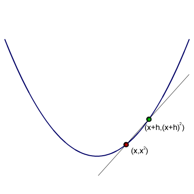
Let's be bold, and try to find the gradient at a general point

A

(x, y) = (x, x^{2})

. To do this, we're going to need another point

B

(x + h, y + k) = (x + h, (x + h)^{2})

. Remember the idea? We're going to find the gradient of the chord between

A

and

B

, and then we're going to let

h

tend to 0 (that is, we'll move

B

closer and closer to

A

) and see whether we can figure out the limit of the gradients.

What is the gradient of the chord

A B

? Well, the chord is just a straight line, so its gradient is (change in

y

)/(change in

x

). The change in

x

is easy: that's just

h

. What about the change in

y

? Well, the

y

-value at

A

x^{2}

, and the

y

-value at

B

(x + h)^{2}

, so the change is

(x + h)^{2} - x^{2} = x^{2} + 2 h x + h^{2} - x^{2} = 2 h x + h^{2}

(multiply out the brackets yourself if you're not sure about this!). So the gradient of the chord

AB

(2 h x + h^{2}) / h = 2 x + h

. So far, so good. Now, as

h

tends to 0, can you see that

2 x + h

is going to tend to

2 x

? So as we move

B

towards

A

, the gradients of the chords tend to

2 x

, so the gradient of the curve at the point

(x, y)

2 x

. And I never got my pencil and ruler out to actually draw some tangents!

Exercise 2: How does this answer compare with your experimentation in Exercise 1?

Now let's try a curve that's a little bit more complicated (but not much): $y = x^{3}$ .

Exercise 3: Repeat Exercise 1, but this time using $y = x^{3}$ .

For this curve, our general point $A$ is going to be $(x, y) = (x, x^{3})$ , and our point $B$ will be $(x + h, y + k) = (x + h, (x + h)^{3})$ . What's the gradient of $A B$ ? The change in $x$ is just $h$ , again.

Exercise 4: By multiplying out the brackets (or using the Binomial Theorem, if you know about this), work out $(x + h)^{3}$ .

This time the change in $x$ is $(x + h)^{3} - x^{3} = x^{3} + 3 h x^{2} + 3 h^{2} x + h^{3} - x^{3} = 3 h x^{2} + 3 h^{2} x + h^{3}$ . So the gradient of $A B$ is $(3 h x^{2} + 3 h^{2} x + h^{3}) / h = 3 x^{2} + 3 h x + h^{2}$ . Now, what happens as $h$ tends to 0? Well, certainly the $h^{2}$ bit is going to tend to 0. (Are you happy with this?) But also, so is the $3 h x$ bit - even if $x$ is quite big, when $h$ gets absolutely tiny, $3 h x$ is going to be pretty small. Try this with some numbers if you don't believe me! So as $h$ tends to 0, the gradient of $A B$ tends to $3 x^{2}$ , so this is the gradient of $y = x^{3}$ at $(x, y)$ .

Exercise 5: Compare this answer with your experimentation in Exercise 3.

Exercise 6: Work out $(x + h)^{4}$ (I promise not to do any more of these, but this one shouldn't be too bad!).

Exercise 7: Using the ideas from above and your answer to Exercise 6, work out the gradient of $y = x^{4}$ at $(x, y)$ .

Exercise 8: Draw up a table like this one:

$y =$ Gradient

$x^{2}$ $2 x$

$x^{3}$

$x^{4}$

$x^{n}$
Fill in the answers you've got so far. Can you spot a pattern? Can you guess what the gradient's going to be for $y = x^{n}$ ?

You may by now have spotted that to do this more generally we're going to need to work out $(x + h)^{n}$ . To do this properly, we'd need the Binomial Theorem. If you're interested, you can read about this on the Maths Thesaurus. I'm not going to go into details about that now; instead, we're going to cheat slightly (but I promise it does work really!). Hopefully you worked out $(x + h)^{3}$ and $(x + h)^{4}$ earlier. Did you notice that we got something of the form $x^{n} + n h x^{n - 1} + h^{2} \times (some other stuff)$ ? (Yes, I know, "some other stuff'' isn't very mathematical, but that's where we'd use the Binomial Theorem if we were being rigorous.) This time, our point $A$ is $(x, y) = (x, x^{n})$ , and our point $B$ is $(x + h, (x + h)^{n})$ . Again, the change in $x$ is $h$ , and when we work out the change in $y$ , we're going to get $(x + h)^{n} - x^{n} = n h x^{n - 1} + h^{2} (some other stuff)$ . So when we work out the gradient of $A B$ , we're going to have $(n h x^{n - 1} + h^{2} (some other stuff)) / h = n x^{n - 1} + h (some other
stuff)$ . Now let's think about what happens as $h$ tends to 0. Well, as we hopefully agreed earlier, $h$ times anything fixed is going to tend to 0 as $h$ tends to 0, and whilst the (some other stuff) isn't actually fixed, the only thing in it that changes is anything involving $h$ , so that's just going to get smaller too. So the gradient of $A B$ tends to $n x^{n - 1}$ as $h$ tends to 0, so the gradient of $y = x^{n}$ is $n x^{n - 1}$ at $(x, y)$ . Does this agree with your guess in Exercise 8?

Exercise 9: Work out the gradients of

y = 2 x^{2}

y = 17 x^{2}

y = - x^{2}

y = a x^{2}

a

y = 2 x^{3}

y = a x^{3}

y = a x^{n}

Exercise 10: What would happen if we tried to work out the gradient of $y = x^{3} + x^{2}$ ? Think carefully about what you'd get if you used the technique above. Now can you work out the gradient of $y = x^{n} + x^{m}$ without really doing any work? (If you need to, start writing it all out, and see whether you can spot how to make it easier.)

Exercise 11: What happens if you use our rule on a straight line $y = a x + b$ ? Does this give the answer you'd expect? What about $y = 7$ , or $y = 15$ ?

Exercise 12: (A little harder) Try using the technique we've used above to work out the gradient of the chord $A B$ on the curve $y = \frac{1}{x}$ , and see whether you can work out the gradient of the curve at $(x, y)$ . How does this compare with the formula? (Note that $y = \frac{1}{x} = x^{- 1}$ , so you can substitute $n = - 1$ into the formula above, although we haven't actually proved that it should work, because we don't know what $(x + h)^{- 1}$ is.)

This technique we've developed to find the gradient of a curve is called differentiation. Hopefully you now understand how to differentiate any polynomial. You don't have to do it from first principles each time: once we've proved the basic results, we can just quote the fact that $a x^{n}$ differentiates to $n a x^{n - 1}$ and so on. It's possible to differentiate other curves too; for example, we could find the gradient of the curves $y = \frac{1}{x^{n}}$ (maybe you've already guessed how to do this), $y = \sin x$ , or $y = 2^{x}$ . However, these require a little bit more technical machinery, so we'll leave them for now.

As a quick aside, let's very briefly mention integration, as it's the `other' part of calculus that comes up at A-level, although we shan't go into any details here. Let's imagine a slightly different scenario: here, we know how fast someone travelled, and how long for, and want to work out how far they went. This time we use

$distance = speed \times time$

(just rearranging the formula from above). This time, we could use a speed-time graph and work out the area under the graph to find the distance. If the lines surrounding the region are all straight, then this isn't too hard - you've probably done questions like this that involve you having to find the areas of triangles, rectangles and trapezia.

But what if the line is curved? You might have come across the idea of approximating the area by roughly splitting it into triangles, rectangles, and trapezia,

but this effectively means pretending that the curve is made up of several straight sections, and this is never going to be precise. We can use integration to find the area under the curve without this approximation.

I've said that we use differentiation to find speed on a distance-time graph, and integration on a speed-time graph. This sort of suggests that they're related - a little bit like the link between addition and subtraction, where we can use one to "undo'' the other. There is a theorem called the Fundamental Theorem of Calculus (sounds impressive, doesn't it?!) that explains this relationship more precisely, and that's why I wanted to mention integration briefly too.

Differentiation (and calculus more generally) is a very important part of mathematics, and comes up in all sorts of places, not only in mathematics but also in physics (and the other sciences), engineering, economics, .... The list goes on!