Copyright © University of Cambridge. All rights reserved.
'Learning Probability Through Mathematical Modelling' printed from https://nrich.maths.org/
Show menu
This article is part of our collection Great Expectations: Probability through Problems.
 I have just read an article called Up and Down the Ladder of Abstraction. Reading it, it occurred to me that the process the author, Bret Victor, is describing can also be applied to our approach to
the teaching and learning of probability. He is talking about how designers should consciously move between concrete systems on the ground, and abstract systems described by equations or statistics.
I have just read an article called Up and Down the Ladder of Abstraction. Reading it, it occurred to me that the process the author, Bret Victor, is describing can also be applied to our approach to
the teaching and learning of probability. He is talking about how designers should consciously move between concrete systems on the ground, and abstract systems described by equations or statistics.
We do the same thing in maths - often called the modelling cycle - and it is one of the fundamentals of our approach to the teaching and learning of probability.
I will illustrate this with our problem Who Is Cheating? In this problem, we want to explore the results of drug testing on athletes who do (not) take a certain banned substance to enhance their performance.
We start with one simulation, and explore that.
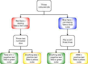 The flow chart on the right (click here for a full size version, or click here for a text version) gives the steps in
carrying out an initial simulation. In the first phase of the simulation, the student takes a blue or red cube depending on the throw of a die. In both cases, the student then follows the appropriate path in the flow chart, ending up with a pair of cubes, one either blue or red, the other either green or yellow.
The flow chart on the right (click here for a full size version, or click here for a text version) gives the steps in
carrying out an initial simulation. In the first phase of the simulation, the student takes a blue or red cube depending on the throw of a die. In both cases, the student then follows the appropriate path in the flow chart, ending up with a pair of cubes, one either blue or red, the other either green or yellow.
Blue means an athlete is not taking a banned substance, red means that the athlete is taking the banned substance. Green means that the result of a test for this substance is negative, yellow that it is positive.
The outcomes at each stage of the simulation are controlled by a die which has four blue sides and two red ones (or if this is not available, an ordinary numbered die, interpreting the outcomes 1 to 4 as blue, and 5 and 6 as red), the sum on two ordinary numbered dice, and a coin flipped three times.
It would be a mistake for a teacher to assume that this first experiment is straightforward for all students - experience would suggest that although some will get the hang of it immediately, others will not. It is therefore good practice with investigations of this nature to do this experiment with the whole class, getting different students to take part. It is important that all students understand how the process works - so when to use which die/dice and when to flip the coin - and what it means - first, is the athlete taking the banned substance (red cube if yes, blue if no), secondly is the test positive (yellow cube if yes, green if no).
It is therefore a good idea to do several single simulations, initially using results as students obtain them through throwing the dice and flipping the coins, but then establishing what would happen for all possible outcomes at each stage, if one or more don't happen without intervention.
Questions that could be asked at this stage include:
But before doing that, students should be coming up with hypotheses about what they think the aggregated data is telling them:
 So far, all we have is experimental data. It may provide fairly convincing evidence for hypotheses, but we need to ask the question - is what we think we see simply a random effect, or are we seeing evidence
for a genuine pattern which we would expect to see more generally in this experiment? While it is important for students to do the practical investigation, it is equally important that they are able to move away from practical results to consider what would happen if we could average the results of an infinite series of experiments - ie. what we expect to
happen.
So far, all we have is experimental data. It may provide fairly convincing evidence for hypotheses, but we need to ask the question - is what we think we see simply a random effect, or are we seeing evidence
for a genuine pattern which we would expect to see more generally in this experiment? While it is important for students to do the practical investigation, it is equally important that they are able to move away from practical results to consider what would happen if we could average the results of an infinite series of experiments - ie. what we expect to
happen.
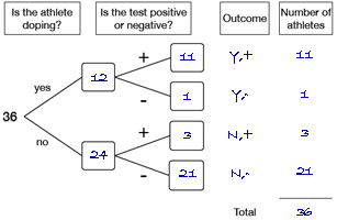
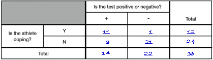 Displaying their results on a tree diagram and 2-way table, and then completing a similar tree diagram and 2-way table for what they would expect to happen, given that they obtained their data by throwing dice and
flipping coins, helps students to compare their practical results with the expected results.
Displaying their results on a tree diagram and 2-way table, and then completing a similar tree diagram and 2-way table for what they would expect to happen, given that they obtained their data by throwing dice and
flipping coins, helps students to compare their practical results with the expected results.
Once students have the tree diagram and 2-way table for the expected results, they can focus on questions such as:
This is the point at which students should be encouraged to progress from expected results in the form of proportions, to probabilities. This is essentially the same calculation, but instead of it being about 36 or 100 or 1000 athletes, proportions are normalised to probabilities - proportions of 1. The total is then the total probability (1) rather than the total number of athletes under consideration.
This is covered in more detail here.
Sooner or later, students should be encouraged to challenge the rules of the simulation. Because the experiment makes use of dice and coins, the proportion of athletes in a given outcome at any stage is pre-determined. How about if we want to be able to change the parameters?
That's where the computer simulation comes in. Not only can it be used to provide much larger data sets quickly, it can also be used to vary the proportions. This provides data to explore questions like:
In Stages 2 and 3, students were encouraged to move away from the practical experiment, using tree diagrams and 2-way tables to explore the theoretical model, and a computer simulation to explore what happens if the parameters are varied.
It is time to revisit the original problem, and the questions and hypotheses which emerged in the early stages. Do answers to these need revising? Can we say more than we could when we just had the experimental results to consider?
Are there questions which have emerged since then? Can we answer them?
Are there any results which seem bizarre or unlikely? For instance, it might be possible to vary the parameters so that either the false positive or negative rate was zero. Is this likely in reality? Is it ever possible for both to be zero at the same time?
The context for this problem was drug-testing among athletes, but this model could be applied to a variety of scenarios. Students could be challenged to set up their own probability model, based on a different scenario, and with rules for the initial simulation defined in a different way.
At its most general, this is a problem about two events, A (athletes taking a banned substance) and B (a test for that substance proving positive), and their complements. The structure of this problem and its analysis could be applied to any context where two events and their complements can be defined, and which make sense in the real world. Students should generalise their analysis for the scenario of A followed by B, then reverse it for the scenario of B followed by A.
Questions which might then be asked include:
I have just read an article called Up and Down the Ladder of Abstraction. Reading it, it occurred to me that the process the author, Bret Victor, is describing can also be applied to our approach to
the teaching and learning of probability. He is talking about how designers should consciously move between concrete systems on the ground, and abstract systems described by equations or statistics.We do the same thing in maths - often called the modelling cycle - and it is one of the fundamentals of our approach to the teaching and learning of probability.
I will illustrate this with our problem Who Is Cheating? In this problem, we want to explore the results of drug testing on athletes who do (not) take a certain banned substance to enhance their performance.
We start with one simulation, and explore that.
Stage 1: the experiment
The flow chart on the right (click here for a full size version, or click here for a text version) gives the steps in
carrying out an initial simulation. In the first phase of the simulation, the student takes a blue or red cube depending on the throw of a die. In both cases, the student then follows the appropriate path in the flow chart, ending up with a pair of cubes, one either blue or red, the other either green or yellow.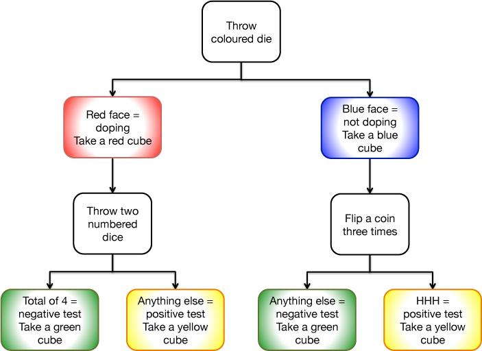
Blue means an athlete is not taking a banned substance, red means that the athlete is taking the banned substance. Green means that the result of a test for this substance is negative, yellow that it is positive.
The outcomes at each stage of the simulation are controlled by a die which has four blue sides and two red ones (or if this is not available, an ordinary numbered die, interpreting the outcomes 1 to 4 as blue, and 5 and 6 as red), the sum on two ordinary numbered dice, and a coin flipped three times.
It would be a mistake for a teacher to assume that this first experiment is straightforward for all students - experience would suggest that although some will get the hang of it immediately, others will not. It is therefore good practice with investigations of this nature to do this experiment with the whole class, getting different students to take part. It is important that all students understand how the process works - so when to use which die/dice and when to flip the coin - and what it means - first, is the athlete taking the banned substance (red cube if yes, blue if no), secondly is the test positive (yellow cube if yes, green if no).
It is therefore a good idea to do several single simulations, initially using results as students obtain them through throwing the dice and flipping the coins, but then establishing what would happen for all possible outcomes at each stage, if one or more don't happen without intervention.
Questions that could be asked at this stage include:
- How many possible outcomes are there?
- Are all outcomes equally likely?
- Why (not)?
But before doing that, students should be coming up with hypotheses about what they think the aggregated data is telling them:
- Does the data aggregated for the whole class convey the same impressions as you obtained from your data? How is it similar, how is it different?
- Are all outcomes equally likely?
- Why (not)?
- Are you surprised at the number of any outcome? There might be more than you intuitively expected, there might be fewer.
- Do you think we would find the same sort of results if we were to do the experiments again?
Stage 2: exploring the model
So far, all we have is experimental data. It may provide fairly convincing evidence for hypotheses, but we need to ask the question - is what we think we see simply a random effect, or are we seeing evidence
for a genuine pattern which we would expect to see more generally in this experiment? While it is important for students to do the practical investigation, it is equally important that they are able to move away from practical results to consider what would happen if we could average the results of an infinite series of experiments - ie. what we expect to
happen. Displaying their results on a tree diagram and 2-way table, and then completing a similar tree diagram and 2-way table for what they would expect to happen, given that they obtained their data by throwing dice and
flipping coins, helps students to compare their practical results with the expected results.Once students have the tree diagram and 2-way table for the expected results, they can focus on questions such as:
- What proportion of the athletes who were taking the banned substance would we expect to test negative?
- What proportion of the athletes who were not taking the banned substance would we expect to test positive?
Stage 3: generalising the method
This is the point at which students should be encouraged to progress from expected results in the form of proportions, to probabilities. This is essentially the same calculation, but instead of it being about 36 or 100 or 1000 athletes, proportions are normalised to probabilities - proportions of 1. The total is then the total probability (1) rather than the total number of athletes under consideration.
This is covered in more detail here.
Stage 4: generalising the problem
Sooner or later, students should be encouraged to challenge the rules of the simulation. Because the experiment makes use of dice and coins, the proportion of athletes in a given outcome at any stage is pre-determined. How about if we want to be able to change the parameters?
That's where the computer simulation comes in. Not only can it be used to provide much larger data sets quickly, it can also be used to vary the proportions. This provides data to explore questions like:
- If the test has a 1% false positive rate and a 0.5% false negative rate, what proportion of athletes would get an incorrect result? How does this vary as the proportion of doping athletes varies?
- If the test will be considered acceptable when not more than 2 in 1000 athletes get an incorrect result, what false positive and negative rates would you recommend?
- Do you think that a false positive is more acceptable than a false negative, or vice versa?
- Ideally we would want them to be zero. Is this going to be possible? If yes, under what conditions?
Stage 5: revisiting the problem
In Stages 2 and 3, students were encouraged to move away from the practical experiment, using tree diagrams and 2-way tables to explore the theoretical model, and a computer simulation to explore what happens if the parameters are varied.
It is time to revisit the original problem, and the questions and hypotheses which emerged in the early stages. Do answers to these need revising? Can we say more than we could when we just had the experimental results to consider?
Are there questions which have emerged since then? Can we answer them?
Are there any results which seem bizarre or unlikely? For instance, it might be possible to vary the parameters so that either the false positive or negative rate was zero. Is this likely in reality? Is it ever possible for both to be zero at the same time?
Stage 6: generalise the problem
The context for this problem was drug-testing among athletes, but this model could be applied to a variety of scenarios. Students could be challenged to set up their own probability model, based on a different scenario, and with rules for the initial simulation defined in a different way.
Stage 7: generalise the questions
At its most general, this is a problem about two events, A (athletes taking a banned substance) and B (a test for that substance proving positive), and their complements. The structure of this problem and its analysis could be applied to any context where two events and their complements can be defined, and which make sense in the real world. Students should generalise their analysis for the scenario of A followed by B, then reverse it for the scenario of B followed by A.
Questions which might then be asked include:
- Do both make sense in the real world?
- Can you derive a general formula for P(A|B)?
- How about P(B|A)?
- How are these two related?