Differential equation questions in STEP and other advanced mathematics examinations come in several forms. Primarily, they can be first order differential equations, i.e. the highest present derivative is the first, or higher order, i.e. there is a derivative larger than the first. Sometimes, the question will lead you through a particular technique for solving the differential equation. More frequently however, you will need to apply a standard technique to solve, and this article covers the two main techniques for first order differential equations. It is worth noting though, that as with most of STEP and other advanced mathematics examinations you should make sure you know all of the differentiation and integration in A-Level very well; that includes importantly implicit differentiation. With that final point in mind though, lets proceed to our first technique, separation of variables.
 

The first technique, for use on first order 'separable' differential equations, is separation of variables. A first order differential equation \(dy/dt\) is said to be separable if it can be written in the form:

\( \hspace{3.25 in} \frac{dy}{dt}=f(y)g(t).\)

Then, separation of variables means to divide through by \(f(y)\) and then integrate with respect to \(t\), i.e.:

\( \hspace{3 in} \int \frac{1}{f(y)}dy = \int g(t)dt.\)

There's really no more to it than that! Though of course the integrals on the left and right hand sides may not be particularly simple ones; they'l often require you to make a substitution. That's one of the reasons why knowing A-Level integration inside out is of key importance; and you should consider going through Module 10 as well for some hints and tips there.
 

Our second technique exploits the product rule for differentiation to solve first order differential equations that can be written in the form:

\( \hspace{3.1 in} \frac{dy}{dt}+p(t)y=f(t).\)

Our aim is to be able to write the left hand side as \( \frac{d}{dt}[g(t)y]\) for some function \(g(t)\). You don't need to worry too much about why, but if we take \(g(t)=e^{\int p(t)dt} \) then we have what we want. \(g\) here is what we usually refer to as our integrating factor. Specifically, this means our steps are:

\( \hspace{1.5 in} \eqalign{ \frac{dy}{dt}+p(t)y &= f(t),
\cr \Rightarrow e^{\int p(t)dt} \frac{dy}{dt} + p(t)e^{\int p(t)dt}y &= e^{\int p(t)dt} f(t),
\cr \Rightarrow \frac{d}{dt} \left[e^{\int p(t)dt} y \right] &= e^{\int p(t)dt} f(t),
\cr \Rightarrow e^{\int p(t)dt} y &= \int e^{\int p(t)dt} f(t)dt,
\cr \Rightarrow y &= \frac{1}{e^{\int p(t)dt}} \int e^{\int p(t)dt} f(t)dt. }  \)

Now, as a hopefully illuminating example, lets take the simple case:

\( \hspace{3.3 in} \frac{dy}{dt}+3y=2.\)

Then our integrating factor is:

\( \hspace{3.35 in} e^{\int 3dt}=e^{3t}.\)

And we have jumping to the final formula above:

\( \hspace{1.8 in} y=\frac{1}{e^{3t}} \left[ \int 2e^{3t}dt \right]=\frac{1}{e^{3t}} \left[\frac{2}{3} e^{3t}+C \right] = \frac{2}{3}+Ce^{-3t}. \)

So, they're the two techniques you'll need to become familiar with to begin to tackle STEP first order differential equation problems. To really test things out though, lets proceed to work through part of a past STEP question.
 

  

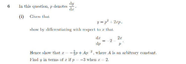
This extract is from Question 6 on STEP III 2008 and it gives a nice introduction to first order differential equations in STEP. Firstly, we're first asked to differentiate \(y\) with respect to \(x\). The import thing to remember is that \(p\) is itself a function of \(x\) and so we're doing implicit differentiation. We find:

\( \hspace{2 in} \frac{dy}{dx}=\frac{d}{dx} \left(p^2+2xp \right)=2p \frac{dp}{dx}+2x \frac{dp}{dx}+2p.\)

Then, realising the LHS \(dy/dx\) can be replaced by \(p\) and rearranging suitabily we find:

\( \hspace{1.85 in} \frac{dp}{dx}=-\frac{p}{2p+2x} \Rightarrow \frac{dx}{dp}=-\frac{(2p+2x)}{p}=-2-2\frac{x}{p}, \)

as required.

So, now we've got ourselves a differential equation for \(x\) that we need to solve. We ask ourselves firstly if it is separable, and the answer should hopefully clearly be no. But, it is of the form that allows us to use integrating factors. This should be a lot clearer if we write it as:

\( \hspace{3.2 in} \frac{dx}{dp}+\frac{2}{p} x=-2. \)

First then, we need to find our integrating factor. Here it is given by:

\( \hspace{2.68 in} e^{\int \frac{2}{p} dp}=e^{2 \ln p}=e^{\ln p^2} = p^2. \)

Therefore multiplying through and proceeding along the steps we went through in general earlier, or jumping to the final formula, we have:

\( \hspace{1.5 in} x=\frac{1}{p^2} \left[ \int -2p^2dp \right] =\frac{1}{p^2} \left[ -\frac{2p^3}{3}+A \right]=-\frac{2}{3}p + A\frac{1}{p^2}, \)

as required. Then our condition \(p=-3\), \(x=2\) gives us \(A\):

\(\hspace{1.7 in} 2=-\frac{2}{3}(-3)+A \frac{1}{(-3)^2} \Rightarrow 2=2+A \frac{1}{9} \Rightarrow A=0. \)

So, we have \(x=-\frac{2}{3}p\) or \(p=-\frac{3}{2}x\), and substituting this in our original equation for \(y\) we have our final answer:

\( \hspace{2.3 in} y=(-\frac{3}{2} x)^2+2x(-\frac{3}{2} x)=-\frac{3}{4} x^2. \)
 

And that, is that! We've covered the two main techniques for tackling first order differential equations in STEP and other advanced mathematics examinations. Hopefully it should be clear that you need to be happy to differentiate and integrate standard expressions easily, and beyond that it's really just a matter of practice with the key techniques. For STEP III in particular though, higher order differential equations arise. To prepare for them, move on to the next article in this module.