Maths and climate change: the melting Arctic

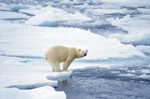
The Arctic sea ice cover is shrinking fast and the potential consequences are grim. To predict how much longer the Arctic sea ice will be around and to assess the impact of an ice-free Arctic, we need to understand how sea ice responds to its environment. Mathematical modelling of sea ice behaviour can provide this much-needed glimpse into the future.

How does ice grow?

How would a slab of sea ice grow if temperature were the only factor to consider?

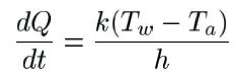
To build a simple model, imagine a round slab of ice of uniform thickness and unit surface area floating on a column of water. Above the ice we have a column of air. We'll assume that the temperatures T$_a$ of air and T$_w$ of water are constant. Now the warmer sea water will transfer energy through the ice into the air above in the form of heat, Q, measured in joules. Fourier's law of heat conduction describes the rate of heat transfer in terms of T$_a$ and T$_w$, the thickness h and the thermal conductivity k of the ice:



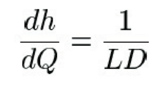
As the sea water below the ice loses heat, a layer on the water surface will freeze. The rate of growth of the thickness of the ice as heat escapes can be expressed in terms of the density D and latent heat L of the sea water:



Combining this with Fourier's equation gives



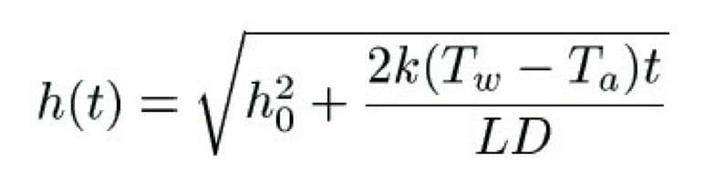
where h$_0$ is the initial thickness of the ice.

The important bit of information in this model is that the ice slab grows with time t like the square root of t. This means that as the ice thickness increases, the rate of growth slows: cracks in the ice will try and “heal” themselves by growing faster than the surrounding thicker ice.  An ice field of varying thickness will try to become level as thin ice grows more rapidly than thick ice.


How does ice move?

But sea ice does not stand still. Winds tear at its surface and it is driven by ocean currents. A simple model of the motion of ice floes is based on Newton's second law of motion, which states that the acceleration of an object is equal to the net force acting on it, divided by the object's mass.

In the case of sea ice, the most important stresses at work are air stress s$_a$, due to wind, water stress s$_w$, due to currents, and the Coriolis force C, due to the motion of the Earth. This gives

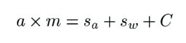
where a is acceleration and m is mass.

It's possible to express the components of this equation in terms of vectors representing the velocities of air, water and ice, taking into account the shape of the ice floe, which determines how it reacts to the currents and the wind. The resulting model predicts that an ice floe moving about unimpeded will eventually move steadily at an angle of about 45 degrees to the right of the wind and at about 3% of the wind speed. Real ice floes have been seen behaving like this.

Any mathematical model is built on observations and its predictions must be compared to real-life data. Gathering data on the thickness and extent of Arctic sea ice involves information from satellites and from submarines that travel under the ice. Analysing the data requires sophisticated statistical methods. But luckily for the members of the Polar Ocean Physics Group at the University of Cambridge, gathering the data means lots of exciting field work in the Arctic!

Reality is of course more complicated than the assumptions underlying the models presented here, but these simple models form the basic building blocks of more sophisticated ones, which themselves feed into global climate models.


This is an edited version of an article written by Dr Marianne Freiberger, based on an interview with Professor Peter Wadhams, Head of the Polar Ocean Physics research group at the University of Cambridge, and published in Plus (plus.maths.org), the free online mathematics magazine. ӬYou can read the full version of the article here.